Weekly Expenditure

How Much Did You Spend Last Week?

Studying Weekly Expenditures

EXPERIMENT OBJECTIVE: To determine whether women have a higher total weekly expenditure than men.

1. Setting up R Packages

# SETUP CHUNK- LIBRARIES
#| label: setup
#| echo: false
#| warning: false
#| message: false

library(tidyverse)

── Attaching core tidyverse packages ──────────────────────── tidyverse 2.0.0 ──
✔ dplyr     1.1.4     ✔ readr     2.1.5
✔ forcats   1.0.0     ✔ stringr   1.5.2
✔ ggplot2   4.0.0     ✔ tibble    3.3.0
✔ lubridate 1.9.4     ✔ tidyr     1.3.1
✔ purrr     1.1.0     
── Conflicts ────────────────────────────────────────── tidyverse_conflicts() ──
✖ dplyr::filter() masks stats::filter()
✖ dplyr::lag()    masks stats::lag()
ℹ Use the conflicted package (<http://conflicted.r-lib.org/>) to force all conflicts to become errors

library(mosaic) # Our all-in-one package

Registered S3 method overwritten by 'mosaic':
  method                           from   
  fortify.SpatialPolygonsDataFrame ggplot2

The 'mosaic' package masks several functions from core packages in order to add 
additional features.  The original behavior of these functions should not be affected by this.

Attaching package: 'mosaic'

The following object is masked from 'package:Matrix':

    mean

The following objects are masked from 'package:dplyr':

    count, do, tally

The following object is masked from 'package:purrr':

    cross

The following object is masked from 'package:ggplot2':

    stat

The following objects are masked from 'package:stats':

    binom.test, cor, cor.test, cov, fivenum, IQR, median, prop.test,
    quantile, sd, t.test, var

The following objects are masked from 'package:base':

    max, mean, min, prod, range, sample, sum

library(skimr) # Looking at data

Attaching package: 'skimr'

The following object is masked from 'package:mosaic':

    n_missing

library(janitor) # Clean the data

Attaching package: 'janitor'

The following objects are masked from 'package:stats':

    chisq.test, fisher.test

library(naniar) # Handle missing data

Attaching package: 'naniar'

The following object is masked from 'package:skimr':

    n_complete

library(visdat) # Visualize missing data
library(tinytable) # Printing Static Tables for our data

Attaching package: 'tinytable'

The following object is masked from 'package:ggplot2':

    theme_void

library(DT) # Interactive Tables for our data
library(crosstable) # Multiple variable summaries

Attaching package: 'crosstable'

The following object is masked from 'package:purrr':

    compact

library(CardioDataSets)
library(vcd)

Loading required package: grid

Attaching package: 'vcd'

The following object is masked from 'package:mosaic':

    mplot

library(ggformula)
library(infer)

Attaching package: 'infer'

The following objects are masked from 'package:mosaic':

    prop_test, t_test

library(broom) # Clean test results in tibble form
library(resampledata) # Datasets from Chihara and Hesterberg's book

Attaching package: 'resampledata'

The following object is masked from 'package:datasets':

    Titanic

library(openintro) # More datasets

Loading required package: airports
Loading required package: cherryblossom
Loading required package: usdata

Attaching package: 'openintro'

The following object is masked from 'package:mosaic':

    dotPlot

The following objects are masked from 'package:lattice':

    ethanol, lsegments

library(visStatistics) # One package to rule them all
library(ggstatsplot)

You can cite this package as:
     Patil, I. (2021). Visualizations with statistical details: The 'ggstatsplot' approach.
     Journal of Open Source Software, 6(61), 3167, doi:10.21105/joss.03167

2. Read Data

money_modified <- money <- readr::read_csv("../data/4-weekly_expenditure.csv")%>%
  # Clean variable names
  janitor::clean_names(case="snake")

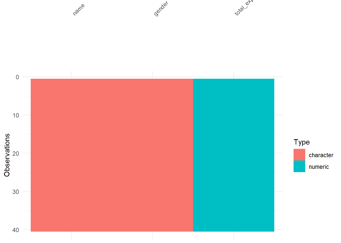
Rows: 40 Columns: 3
── Column specification ────────────────────────────────────────────────────────
Delimiter: ","
chr (2): Name, Gender
dbl (1): Total_Expenditure_Last_Week

ℹ Use `spec()` to retrieve the full column specification for this data.
ℹ Specify the column types or set `show_col_types = FALSE` to quiet this message.

money_modified

# A tibble: 40 × 3
   name      gender total_expenditure_last_week
   <chr>     <chr>                        <dbl>
 1 Radha     Female                        2000
 2 Prerana   Female                        1200
 3 Chris     Male                         15000
 4 Nireeksha Female                        3620
 5 Supraj    Male                           560
 6 Adit      Male                          2200
 7 Shweta    Female                        1500
 8 Diya      Female                        1206
 9 Kshama    Female                        1400
10 Savannah  Female                        2500
# ℹ 30 more rows

3. Examine Data

dplyr::glimpse(money_modified)

Rows: 40
Columns: 3
$ name                        <chr> "Radha", "Prerana", "Chris", "Nireeksha", …
$ gender                      <chr> "Female", "Female", "Male", "Female", "Mal…
$ total_expenditure_last_week <dbl> 2000.0, 1200.0, 15000.0, 3620.0, 560.0, 22…

skimr::skim(money_modified)

Data summary

Name	money_modified
Number of rows	40
Number of columns	3
_______________________
Column type frequency:
character	2
numeric	1
________________________
Group variables	None

Variable type: character

skim_variable	n_missing	complete_rate	min	max	empty	n_unique	whitespace
name	0	1	4	9	0	40	0
gender	0	1	4	6	0	2	0

Variable type: numeric

skim_variable	n_missing	complete_rate	mean	sd	p0	p25	p50	p75	p100	hist
total_expenditure_last_week	0	1	4833.37	8520.35	365	1204.5	2350	4475	50000	▇▁▁▁▁

names(money_modified)

[1] "name"                        "gender"                     
[3] "total_expenditure_last_week"

visdat::vis_dat(money, sort_type = TRUE, palette = "default")

money_modified <- money %>% tidyr::drop_na()
money_modified

# A tibble: 40 × 3
   name      gender total_expenditure_last_week
   <chr>     <chr>                        <dbl>
 1 Radha     Female                        2000
 2 Prerana   Female                        1200
 3 Chris     Male                         15000
 4 Nireeksha Female                        3620
 5 Supraj    Male                           560
 6 Adit      Male                          2200
 7 Shweta    Female                        1500
 8 Diya      Female                        1206
 9 Kshama    Female                        1400
10 Savannah  Female                        2500
# ℹ 30 more rows

visdat::vis_dat(money_modified, sort_type = TRUE, palette = "default")

money_modified %>%
  dplyr::summarise(across(
    .cols = c(total_expenditure_last_week), # select columns

    .fns = list(
      mean = ~ mean(., na.rm = T),
      sd = sd,
      min = min, max = max
    )
  )) %>% 
  tt()

total_expenditure_last_week_mean	total_expenditure_last_week_sd	total_expenditure_last_week_min	total_expenditure_last_week_max
4833.373	8520.354	365	50000

money_modified <- money %>%
  dplyr::mutate(across(where(is.character), as.factor)) %>% 
  relocate(where(is.factor))
glimpse(money_modified)

Rows: 40
Columns: 3
$ name                        <fct> Radha, Prerana, Chris, Nireeksha, Supraj, …
$ gender                      <fct> Female, Female, Male, Female, Male, Male, …
$ total_expenditure_last_week <dbl> 2000.0, 1200.0, 15000.0, 3620.0, 560.0, 22…

money_modified %>%
  stats::setNames(c("Name", "Gender", "Total_Expenditure_Last_Week"))

# A tibble: 40 × 3
   Name      Gender Total_Expenditure_Last_Week
   <fct>     <fct>                        <dbl>
 1 Radha     Female                        2000
 2 Prerana   Female                        1200
 3 Chris     Male                         15000
 4 Nireeksha Female                        3620
 5 Supraj    Male                           560
 6 Adit      Male                          2200
 7 Shweta    Female                        1500
 8 Diya      Female                        1206
 9 Kshama    Female                        1400
10 Savannah  Female                        2500
# ℹ 30 more rows

money_modified %>%
  DT::datatable(
    style = "default",
    caption = htmltools::tags$caption(
      style = "caption-side: top; text-align: left; color: black; font-size: 100%;", "Weekly Expenditure Dataset (Clean)"
    ),
    options = list(pageLength = 10, autoWidth = TRUE)
  ) %>%
  DT::formatStyle(
    columns = names(money_modified),
    fontFamily = "Roboto Condensed",
    fontSize = "12px",
  )

4. Data Dictionary

Qualitative Data

1. name(fct): Name of the student
2. gender(fct): Gender of the student

Quantitative Data

1. total_expenditure_last_week(dbl): Total expenditure of the student the previous week (in Rupees)

5. Graphs

1. Which gender has a higher weekly expenditure?

money_modified2 <- money %>%
  group_by(gender) %>%
  summarise(average_expenditure = mean(total_expenditure_last_week, na.rm = TRUE))

money_modified2 %>% 
  gf_col(average_expenditure ~ gender,
         fill = ~ gender) %>%
  gf_labs(title = "Which gender has a higher weekly expenditure?",
          x = "Gender",
          y = "Average Weekly Expenditure",
          fill = "Legend: Gender") %>% 
  gf_refine(scale_fill_brewer(palette = "Pastel1"))

Inferences

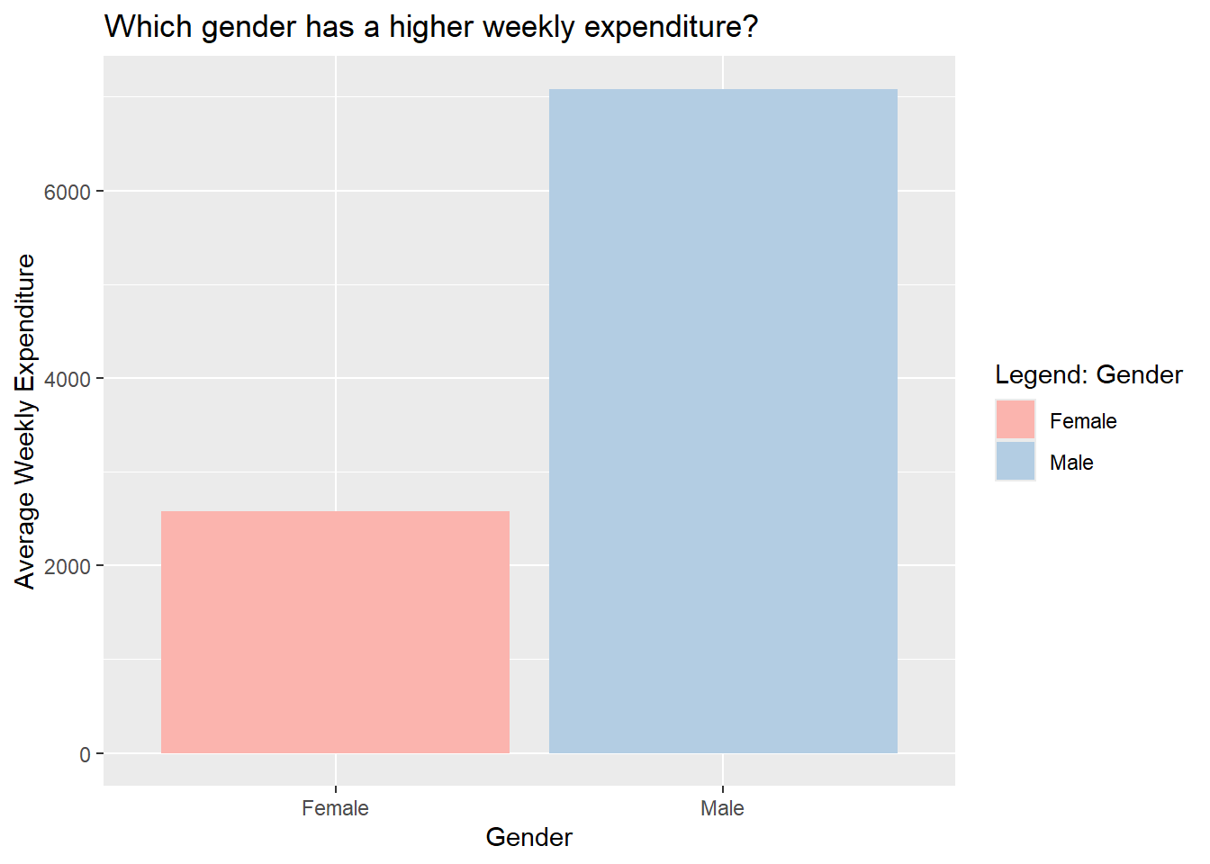
While we surveyed people and told them our objective, a lot of them assumed that women would have a higher weekly expenditure. But clearly, from the data we can tell that men have a much higher average weekly expenditure than women.

One of the men we surveyed mentioned that he bought an electronic device the previous week, which is why his expenditure was so high (50,000). Perhaps if we had surveyed different men, the data would be comparable.

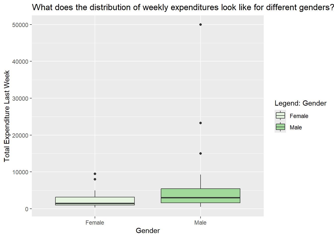
2. What does the distribution of weekly expenditures look like for different genders?

money_modified %>%
  gf_boxplot(total_expenditure_last_week ~ gender,
             fill = ~gender,
             orientation = 'x') %>%
  gf_labs(title = "What does the distribution of weekly expenditures look like for different genders?",
          x = "Gender",
          y = "Total Expenditure Last Week",
          fill = "Legend: Gender") %>% 
  gf_refine(scale_fill_brewer(palette = "Greens"))

Inferences

Men, on average, tend to spend more than women, and there is greater variability in their spending habits, mainly because of the few men with very high expenditures. Female spending is generally more concentrated at the lower end, with fewer extreme high spenders.

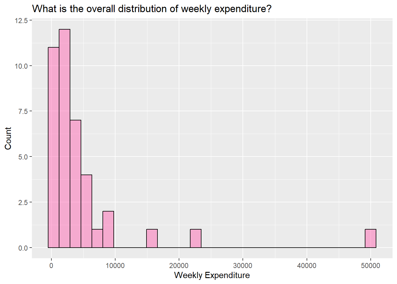
3. What is the overall distribution of weekly expenditure?

money%>% 
gf_histogram(~ total_expenditure_last_week,
             data = money_modified,
             fill = "#ff69b4", 
             color = "black") %>%
  gf_labs(title = "What is the overall distribution of weekly expenditure?",
          x = "Weekly Expenditure",
          y = "Count")

`stat_bin()` using `bins = 30`. Pick better value `binwidth`.

Inferences

It is evident from the graph that the data is highly skewed. Most of the values are concentrated towards the lower end, with a few exceptions of extremely high values. Most expenditures lie between 0-10,000.

6. Summary of Inferences

People initially expected women to spend more, but the data shows the opposite- men have a higher average weekly expenditure. This result is influenced by a few male outliers, including one who spent 50,000 on an electronic device. Because of these extreme values, men’s spending shows much greater variability, while women’s spending remains more consistent and lower overall. The distribution is highly skewed, with most students spending between 0–10,000 and only a few reporting very high expenses. If the sample included different participants, the averages might look more similar.

7. Surprising Aspects

Even if we didn’t consider that one man who spent 50,000, the expenditures of other men were also significantly higher than that of women. What’s funny is that, almost all women were a little hesitant to tell us their expenditure, considering that it was too high and they felt a bit ashamed. Men on the other hand were more open with sharing their details, even though they were at least 3,000-4,000 more than what the women had said. Perhaps we could conclude another thing, that women are more conscious about their spending than men.

8. T test- Inference for a single mean

stats::shapiro.test(x = money_modified$total_expenditure_last_week) %>%
  broom::tidy()

# A tibble: 1 × 3
  statistic  p.value method                     
      <dbl>    <dbl> <chr>                      
1     0.480 9.90e-11 Shapiro-Wilk normality test

library(nortest)
# Especially when we have >= 5000 observations
nortest::ad.test(x = money_modified$total_expenditure_last_week) %>%
  broom::tidy()

# A tibble: 1 × 3
  statistic  p.value method                         
      <dbl>    <dbl> <chr>                          
1      6.71 9.33e-17 Anderson-Darling normality test

The distribution of the total expenditure of students from the previous week is significantly different from a normal distribution.

# t-test
money_ttest <- mosaic::t_test(
  money_modified$total_expenditure_last_week, # Name of variable
  mu = 0, # belief
  alternative = "two.sided"
) %>% # Check both sides
  broom::tidy()
money_ttest

# A tibble: 1 × 8
  estimate statistic  p.value parameter conf.low conf.high method    alternative
     <dbl>     <dbl>    <dbl>     <dbl>    <dbl>     <dbl> <chr>     <chr>      
1    4833.      3.59 0.000918        39    2108.     7558. One Samp… two.sided  

Since the p-value = 0.0009184396 is much smaller than 0.05, we reject the null hypothesis. The 95% confidence interval ([2108.431, 7558.314]) does not include 0. Thus, we can conclude that the average expenditure is significantly greater than 0.