── Attaching core tidyverse packages ──────────────────────── tidyverse 2.0.0 ──
✔ dplyr     1.1.4     ✔ readr     2.1.5
✔ forcats   1.0.0     ✔ stringr   1.5.2
✔ ggplot2   4.0.0     ✔ tibble    3.3.0
✔ lubridate 1.9.4     ✔ tidyr     1.3.1
✔ purrr     1.1.0
── Conflicts ────────────────────────────────────────── tidyverse_conflicts() ──
✖ dplyr::filter() masks stats::filter()
✖ dplyr::lag()    masks stats::lag()
ℹ Use the conflicted package (<http://conflicted.r-lib.org/>) to force all conflicts to become errors
library(mosaic) # Our all-in-one package
Registered S3 method overwritten by 'mosaic':
  method                           from
  fortify.SpatialPolygonsDataFrame ggplot2

The 'mosaic' package masks several functions from core packages in order to add
additional features.  The original behavior of these functions should not be affected by this.

Attaching package: 'mosaic'

The following object is masked from 'package:Matrix':

    mean

The following objects are masked from 'package:dplyr':

    count, do, tally

The following object is masked from 'package:purrr':

    cross

The following object is masked from 'package:ggplot2':

    stat

The following objects are masked from 'package:stats':

    binom.test, cor, cor.test, cov, fivenum, IQR, median, prop.test,
    quantile, sd, t.test, var

The following objects are masked from 'package:base':

    max, mean, min, prod, range, sample, sum
library(skimr) # Looking at data
Attaching package: 'skimr'

The following object is masked from 'package:mosaic':

    n_missing
library(janitor) # Clean the data
Attaching package: 'janitor'

The following objects are masked from 'package:stats':

    chisq.test, fisher.test
library(naniar) # Handle missing data
Attaching package: 'naniar'

The following object is masked from 'package:skimr':

    n_complete
library(visdat) # Visualise missing datalibrary(tinytable) # Printing Static Tables for our data
Attaching package: 'tinytable'

The following object is masked from 'package:ggplot2':

    theme_void
Rows: 40 Columns: 3
── Column specification ────────────────────────────────────────────────────────
Delimiter: ","
chr (3): Name, Gender, Tattoo_Attractive

ℹ Use `spec()` to retrieve the full column specification for this data.
ℹ Specify the column types or set `show_col_types = FALSE` to quiet this message.
tattoo_modified
# A tibble: 40 × 3
   name    gender tattoo_attractive
   <chr>   <chr>  <chr>
 1 Aadya   F      Yes
 2 Abhinav M      Yes
 3 Aditya  M      No
 4 Akash   M      Yes
 5 Amit    M      No
 6 Amogh   M      Yes
 7 Anurag  M      Yes
 8 Arnav   M      Yes
 9 Aryan   M      Yes
10 Ashmita F      No
# ℹ 30 more rows
Rows: 40
Columns: 3
$ name              <fct> Aadya, Abhinav, Aditya, Akash, Amit, Amogh, Anurag, …
$ gender            <fct> F, M, M, M, M, M, M, M, M, F, M, F, M, F, M, F, F, M…
$ tattoo_attractive <fct> Yes, Yes, No, Yes, No, Yes, Yes, Yes, Yes, No, Yes, …
# A tibble: 40 × 3
   Name    Gender Are_Tattoos_Attractive
   <fct>   <fct>  <fct>
 1 Aadya   F      Yes
 2 Abhinav M      Yes
 3 Aditya  M      No
 4 Akash   M      Yes
 5 Amit    M      No
 6 Amogh   M      Yes
 7 Anurag  M      Yes
 8 Arnav   M      Yes
 9 Aryan   M      Yes
10 Ashmita F      No
# ℹ 30 more rows
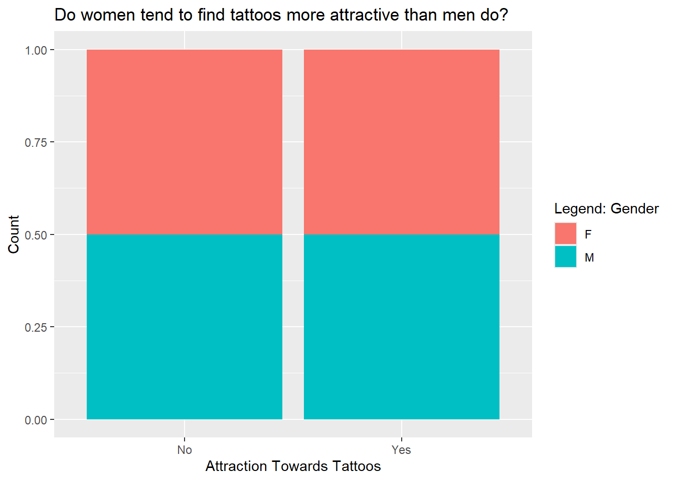
tattoo_modified %>%gf_bar(~tattoo_attractive, fill =~gender, position ="fill") %>%gf_labs(title ="Do women tend to find tattoos more attractive than men do?",x ="Attraction Towards Tattoos",y ="Count",fill ="Legend: Gender")
Inferences
From this sample, it is evident that the number of women who like and dislike tattoos are equal to the number of men who like and dislike tattoos. However, it is possible that a correlation could be found if the sample was different.
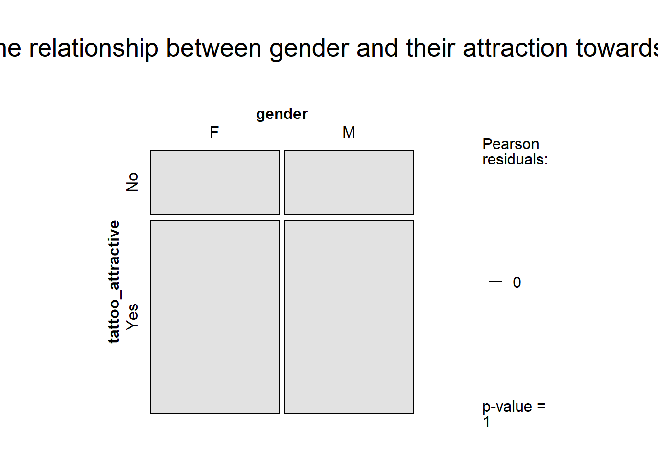
2. What is the relationship between gender and their attraction towards tattoos?
                 gender
tattoo_attractive  F  M Sum
              No   5  5  10
              Yes 15 15  30
              Sum 20 20  40
vcd::structable(gender ~ tattoo_attractive, data = tattoo_modified) %>% vcd::mosaic(gp = shading_max,main ="What is the relationship between gender and their attraction towards tattoos?")
Warning in legend(residuals, gpfun, residuals_type): All residuals are zero.
Inferences
From this particular sample, there is no correlation between gender and their attraction towards tattoos because the number of women who like and dislike tattoos are equal to the number of men who like and dislike tattoos (by coincidence).
There is no colour in the mosaic graph because the data fits the expected model perfectly. There is no difference between genders. The proportions are identical:
15/20 Females = 75% Yes 15/20 Males = 75% Yes
So there is zero association between gender and tattoo preference in your sample, hence zero residuals.
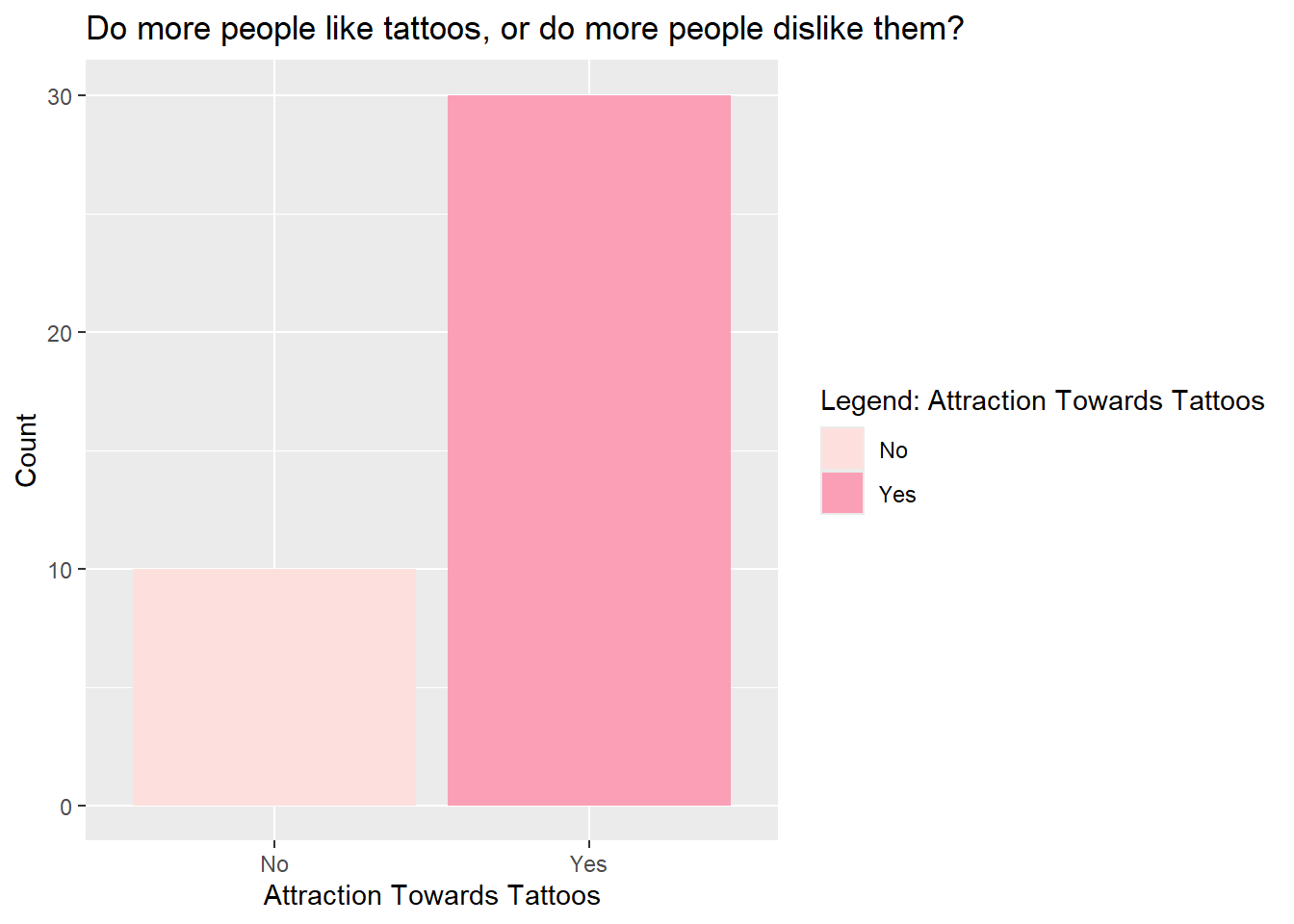
3. Do more people like tattoos, or do more people dislike them?
tattoo_modified %>%gf_bar(~ tattoo_attractive, fill =~tattoo_attractive) %>%gf_labs(title ="Do more people like tattoos, or do more people dislike them? ",x ="Attraction Towards Tattoos",y ="Count",fill ="Legend: Attraction Towards Tattoos") %>%gf_refine(scale_fill_brewer(palette ="RdPu"))
Inferences
Out of the 40 students who were surveyed, 30 of them find tattoos attractive, while 10 of them do not. Clearly, students are more likely to like tattoos than dislike them.
6. Summary of Inferences
From this sample of 40 students, 30 reported finding tattoos attractive and 10 did not, indicating that students are generally more likely to like tattoos than dislike them.
The proportions of males and females who find tattoos attractive are identical (75% each), meaning there is no difference in tattoo preference between genders in this dataset. The mosaic plot shows no colour variation because the observed proportions match the expected proportions perfectly. Therefore, there is no evidence of any association between gender and tattoo preference in this sample. The result appears to be coincidental rather than indicative of a real relationship.
7. Surprising Aspects
It is surprising to see that the data is proportionate. Not much can be inferred from this data sample. I am curious to see how the graphs would change with a different sample.
8. Binom test- Inference test for a single proportion
Null hypothesis: 50% of the students find tattoos attractive. Alternative hypothesis: The proportion of students who find tattoos attractive is either less than or more than 50%.
mosaic::binom.test(~ tattoo_attractive, data = tattoo_modified, success ="Yes")
data:  tattoo_modified$tattoo_attractive  [with success = Yes]
number of successes = 30, number of trials = 40, p-value = 0.002221
alternative hypothesis: true probability of success is not equal to 0.5
95 percent confidence interval:
 0.5880380 0.8730852
sample estimates:
probability of success
                  0.75
mosaic::binom.test(~ tattoo_attractive, data = tattoo_modified, success ="Yes") %>% broom::tidy()
From the binomial test, we can conclude that the estimate value for this sample = 0.75, and that based on this, the population proportion of those who find tattoos attractive is also not 0.5, since the p-value is 0.002221434. So we reject the NULL hypothesis and accept the alternative hypothesis, that the proportion is not 0.5 and more like 0.75.