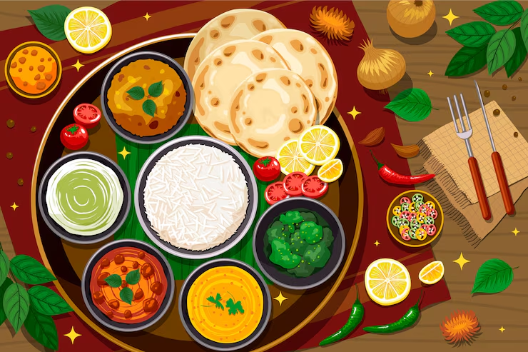
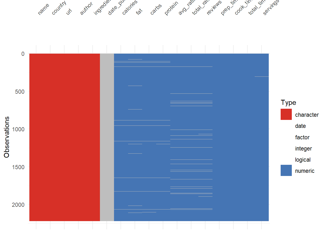
Rows: 2,218
Columns: 17
$ name <fct> "Saganaki (Flaming Greek Cheese)", "Coney Island Knishe…
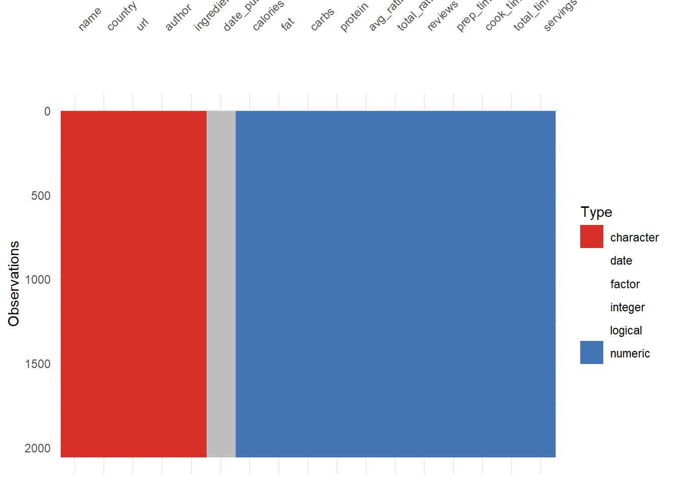
$ country <fct> Greek, Jewish, Australian and New Zealander, Chilean, T…
$ url <fct> https://www.allrecipes.com/recipe/263750/flaming-greek-…
$ author <fct> "John Mitzewich", "John Mitzewich", "CHIPPENDALE", "Hei…
$ ingredients <fct> "1 (4 ounce) package kasseri cheese, 1 tablespoon water…
$ date_published <date> 2024-02-07, 2024-11-26, 2022-07-14, 2025-01-31, 2025-0…
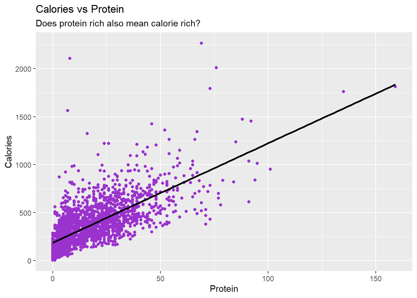
$ calories <dbl> 391, 301, 64, 106, 449, 958, 378, 90, 157, 322, 4, NA, …
$ fat <dbl> 25, 17, 3, 9, 23, 24, 10, 5, 6, 16, 0, NA, 21, 2, 66, 8…
$ carbs <dbl> 15, 31, 9, 7, 58, 144, 59, 10, 25, 39, 1, NA, 16, 63, 7…
$ protein <dbl> 16, 7, 1, 1, 7, 46, 14, 1, 2, 7, 0, NA, 28, 6, 54, 17, …
$ avg_rating <dbl> 4.8, 4.6, 4.3, 5.0, 3.8, 4.4, 4.3, NA, 4.6, 5.0, 4.7, 4…
$ total_ratings <dbl> 25, 10, 126, 1, 13, 40, 3, NA, 65, 2, 182, 2, 19, 16, 9…
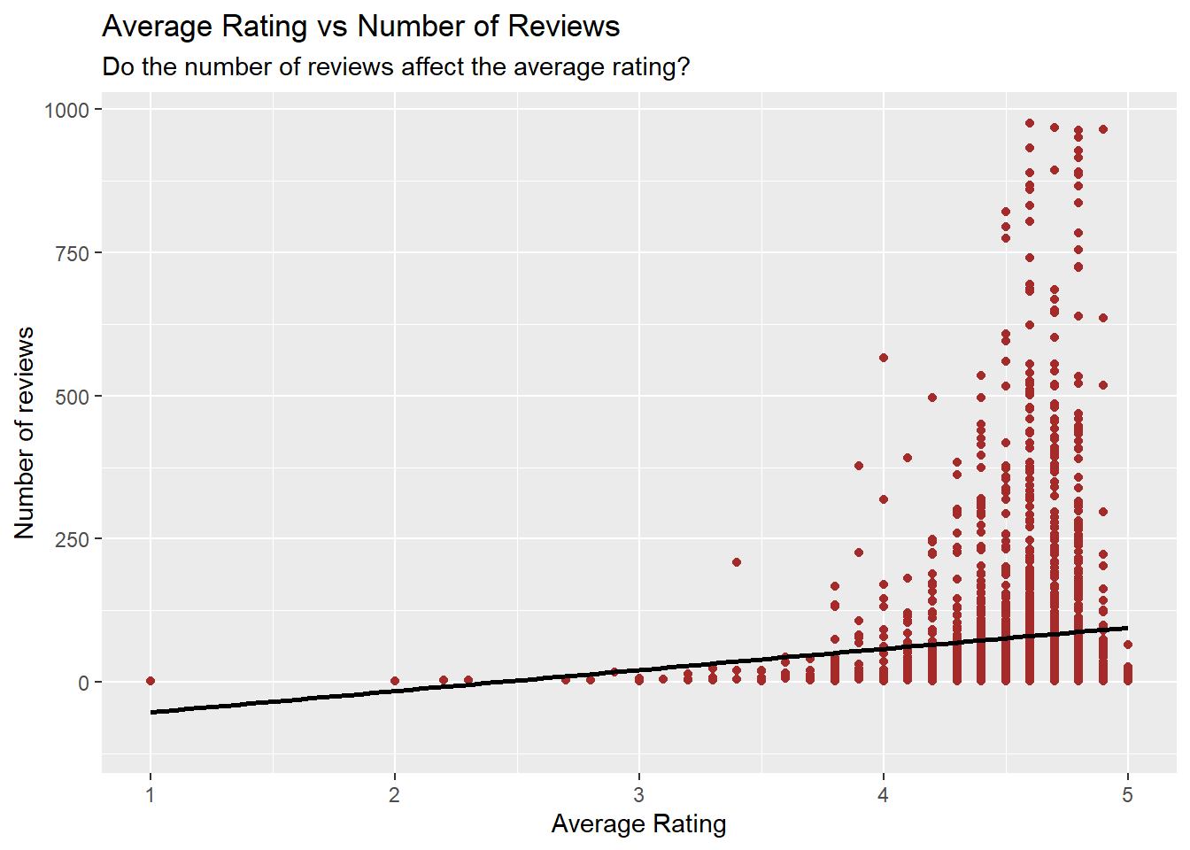
$ reviews <dbl> 22, 9, 104, 1, 11, 32, 3, NA, 55, 2, 138, 2, 15, 16, 84…
$ prep_time <dbl> 10, 30, 20, 10, 30, 30, 30, 40, 0, 5, 5, 5, 10, 10, 20,…
$ cook_time <dbl> 5, 75, 15, 0, 15, 165, 75, 30, 0, 5, 0, 25, 10, 50, 16,…
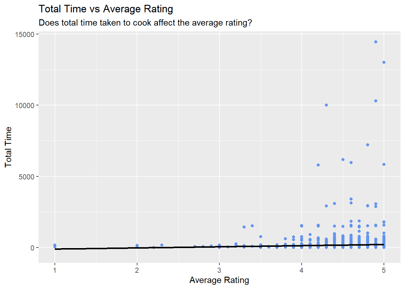
$ total_time <dbl> 15, 180, 180, 10, 45, 675, 585, 155, 0, 10, 5, 30, 50, …
$ servings <dbl> 2, 16, 12, 6, 15, 6, 6, 84, 24, 1, 21, 8, 4, 10, 4, 8, …