── Attaching core tidyverse packages ──────────────────────── tidyverse 2.0.0 ──
✔ dplyr     1.1.4     ✔ readr     2.1.5
✔ forcats   1.0.0     ✔ stringr   1.5.2
✔ ggplot2   4.0.0     ✔ tibble    3.3.0
✔ lubridate 1.9.4     ✔ tidyr     1.3.1
✔ purrr     1.1.0
── Conflicts ────────────────────────────────────────── tidyverse_conflicts() ──
✖ dplyr::filter() masks stats::filter()
✖ dplyr::lag()    masks stats::lag()
ℹ Use the conflicted package (<http://conflicted.r-lib.org/>) to force all conflicts to become errors
library(mosaic) # Our all-in-one package
Registered S3 method overwritten by 'mosaic':
  method                           from
  fortify.SpatialPolygonsDataFrame ggplot2

The 'mosaic' package masks several functions from core packages in order to add
additional features.  The original behavior of these functions should not be affected by this.

Attaching package: 'mosaic'

The following object is masked from 'package:Matrix':

    mean

The following objects are masked from 'package:dplyr':

    count, do, tally

The following object is masked from 'package:purrr':

    cross

The following object is masked from 'package:ggplot2':

    stat

The following objects are masked from 'package:stats':

    binom.test, cor, cor.test, cov, fivenum, IQR, median, prop.test,
    quantile, sd, t.test, var

The following objects are masked from 'package:base':

    max, mean, min, prod, range, sample, sum
library(skimr) # Looking at data
Attaching package: 'skimr'

The following object is masked from 'package:mosaic':

    n_missing
library(janitor) # Clean the data
Attaching package: 'janitor'

The following objects are masked from 'package:stats':

    chisq.test, fisher.test
library(naniar) # Handle missing data
Attaching package: 'naniar'

The following object is masked from 'package:skimr':

    n_complete
library(visdat) # Visualise missing datalibrary(tinytable) # Printing Static Tables for our data
Attaching package: 'tinytable'

The following object is masked from 'package:ggplot2':

    theme_void
Attaching package: 'crosstable'

The following object is masked from 'package:purrr':

    compact
library(vcd)
Loading required package: grid

Attaching package: 'vcd'

The following object is masked from 'package:mosaic':

    mplot
library(visStatistics) # One package to test them all### Dataset from Chihara and Hesterberg's book (Second Edition)library(resampledata)
Attaching package: 'resampledata'

The following object is masked from 'package:datasets':

    Titanic
2. Reading and Cleaning Data
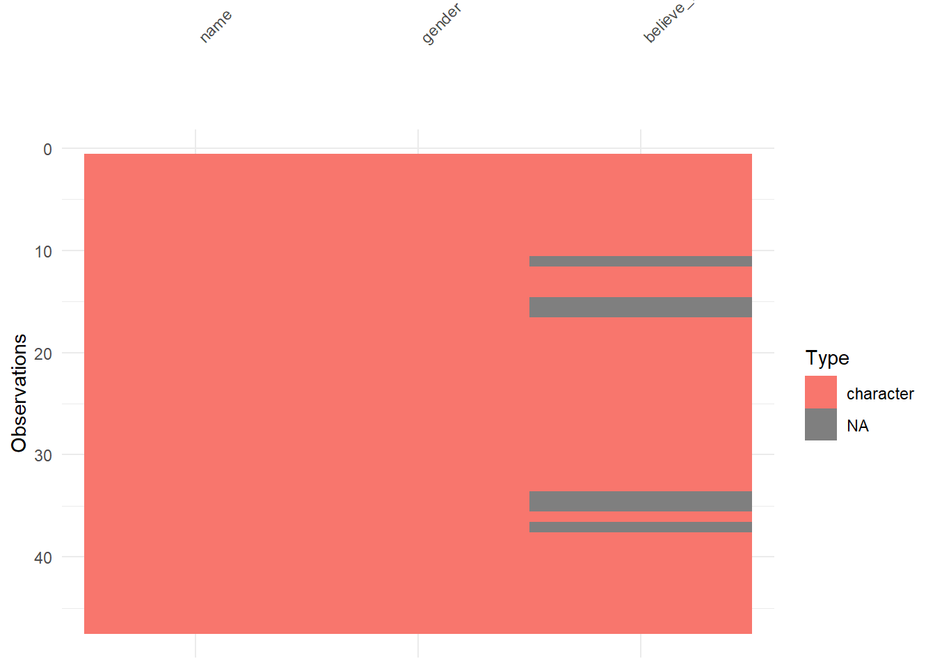
god_modified <- god <- readr::read_csv("../data/5-believe_in_god.csv")%>%# Clean variable names janitor::clean_names(case="snake")
Rows: 47 Columns: 3
── Column specification ────────────────────────────────────────────────────────
Delimiter: ","
chr (3): Name, Gender, Believe_in_God

ℹ Use `spec()` to retrieve the full column specification for this data.
ℹ Specify the column types or set `show_col_types = FALSE` to quiet this message.
god_modified
# A tibble: 47 × 3
   name      gender believe_in_god
   <chr>     <chr>  <chr>
 1 Sanjana   Female Yes
 2 Tathasthu Male   Yes
 3 Vaibhav   Male   Yes
 4 Siddharth Male   Yes
 5 Ashik     Male   No
 6 Kshirab   Female Yes
 7 Niyosha   Female Yes
 8 Charvi    Female No
 9 Anoti     Female Yes
10 Dhruv     Male   No
# ℹ 37 more rows
        believe_in_god
gender   No Yes Sum
  Female  5  18  23
  Male   10   8  18
  Sum    15  26  41
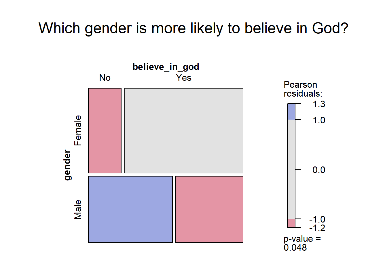
vcd::structable(believe_in_god ~ gender, data = god_modified) %>% vcd::mosaic(gp = shading_max,main ="Which gender is more likely to believe in God?")
Inferences
Females are more likely to believe in God than males. 18/23 women believe in God, whereas only 8/18 men believe in God which is surprisingly less.
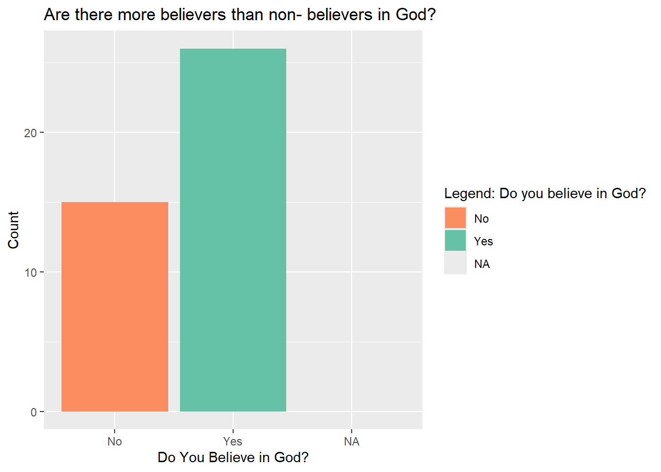
2. Are there more believers than non- believers in God?
god_modified %>%gf_bar(~ believe_in_god, fill =~ believe_in_god) %>%gf_labs( title ="Are there more believers than non- believers in God?",x ="Do You Believe in God?",y ="Count",fill ="Legend: Do you believe in God?") %>%gf_refine(scale_fill_brewer(palette ="Set2", direction =-1))
Inferences
It is evident from the graph that students are more likely to believe in God. The ratio of students who believe vs do not believe in God is almost 2:1.
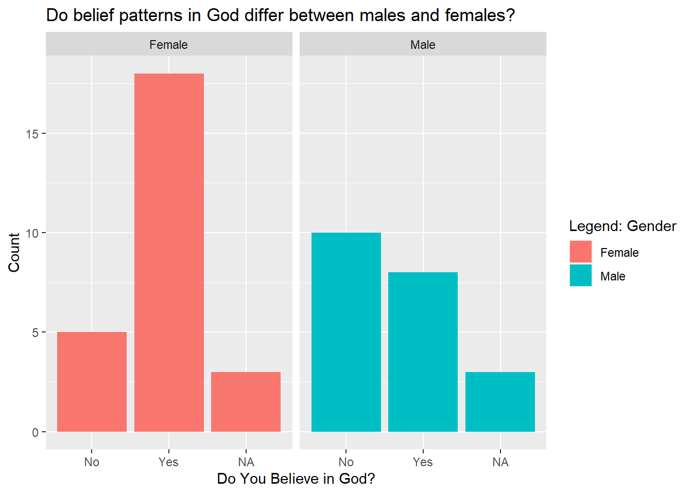
3. Do belief patterns in God differ between males and females?
god_modified %>%gf_bar(~ believe_in_god | gender, fill =~gender) %>%gf_labs( title ="Do belief patterns in God differ between males and females?",x ="Do You Believe in God?",y ="Count",fill ="Legend: Gender")
Inferences
As mentioned before, Females are more likely to believe in God than males. The ratio of female believers to non- believers is almost 3.5:1, while for men it is even less than 2:1.
6. Summary of Inferences
More students believe in God than not, with roughly a 2:1 ratio overall. However, this belief is noticeably stronger among women- around 18 out of 23 females believe in God, compared to only 8 out of 18 males. Female students show a much higher believer-to-non-believer ratio (about 3.5:1), while for males it is under 2:1. Overall, belief in God is more common, and significantly more prevalent among women than men.
7. Surprising Aspects
It is surprising how so many men do not believe in God. When we look at the graph of believers vs non-believers, there are clearly more believers, but 18 of them are women and only 8 of them are men.
8. Binom test- Inference test for a single proportion
Null hypothesis: 50% of the students believe in God. Alternative hypothesis: The proportion of students who believe in God is either less than or more than 50%.
mosaic::binom.test(~ believe_in_god, data = god_modified, success ="Yes")
data:  god_modified$believe_in_god  [with success = Yes]
number of successes = 26, number of trials = 41, p-value = 0.1173
alternative hypothesis: true probability of success is not equal to 0.5
95 percent confidence interval:
 0.4693625 0.7787721
sample estimates:
probability of success
             0.6341463
mosaic::binom.test(~ believe_in_god, data = god_modified, success ="Yes") %>% broom::tidy()
From the binomial test, we can conclude that the estimate value for this sample = 0.6341463, and that based on this, the population proportion of those who find tattoos attractive is also not 0.5, since the p-value is 0.1172752. So we reject the NULL hypothesis and accept the alternative hypothesis, that the proportion is not 0.5 and more like 0.6341463